
Last week I gave a couple of talks at the Pensions, Risk and Investment Conference, organised by the Institute and Faculty of Actuaries. One of them was based on a recent paper I wrote* on pension scheme funding. The talk seemed to strike a chord with many of the pensions professionals there, so I thought I’d share some of the key points here.
Rationale for the paper
The purpose of the paper was threefold. First, it aimed to show that “traditional” valuation approaches were no longer appropriate for pension schemes; second, it explained why, if a more appropriate approach was used, corporate bonds looked like a particularly attractive asset class; and third, it demonstrated that this approach could still be adapted to fit with current regulatory requirements on pension scheme valuations.
A brief history of valuation approaches
To understand why traditional approaches to pension scheme valuation are no longer appropriate, it is helpful to understand why they once were – and why they continue to be appropriate for many purposes. A traditional valuation approach is one that involves calculating a present value of liabilities and comparing it with a value of assets (market or otherwise).
For accounting purposes, this present value approach makes sense – valuations here are intended to given an idea of the impact of a pension scheme on a company’s value, so there is no real alternative to using present values. Similarly, for either buyout valuations or calculations of the Pension Protection Fund levy, the calculation of a premium is needed. This, again, implies a present value approach.
For funding, too, this approach used to be appropriate – when pension schemes were open to future accrual. Here, the main focus of the valuation was on the level of contributions needed to cover accruing benefits. This contribution then needed to be adjusted for any previous over- or under-payment – so values of assets and liabilities were needed.
However, few schemes these days have future benefits being earned to any significant degree. As such, the main question should be more about whether the assets the scheme has are sufficient to cover the pension promises it has made.
A better way
If a pension scheme is aiming for buyout, then the present value approach is still appropriate. However, many pension schemes wish to stay outside the insurance regulatory framework and to aim instead for “self sufficiency”. This is defined in various ways, but can be taken to mean broadly that the intention is for the assets held to pay the liabilities due for the foreseeable future. So success could be defined has having enough assets to outlast the liabilities. If this is the case, why not use a valuation approach that reflects this?
The approach recommended in the paper is the chance of ultimate excess, or “CUE”. This is essentially the likelihood that there will be assets left over once the last pension has been paid. The diagram below shows how this can be calculated. First, we take the liability cash flows, shown in the top left panel. These are the payments that the scheme has to make. In this example, they are assumed to be fixed and known exactly. Neither of these features will be true in real life, but this simplification helps to get the concept of the CUE across. Next, we take the assets and project them forward stochastically. Each period, pension payments will be deducted from the assets. This is represented in the bottom left panel. Because there is uncertainty over what return the assets will give, there is a “funnel of doubt”. Specifically, sometimes there are assets left over when the liabilities have been paid, and sometimes the assets run out before the liabilities have been paid. The distribution of excess amounts is shown in the right hand panel.
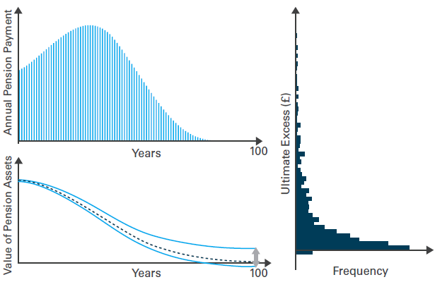
Source: LGIM
As well as seeming more intuitively appropriate for a pension scheme seeking self sufficiency, this approach has other advantages. First, it is possible to look for the asset allocation that maximises the CUE. This is a change from traditional approaches, where there is a wide choice of “efficient” portfolios, requiring either a utility function or some sort of judgement call on which is best for the scheme. Second, it allows not only for differing expected returns but also for volatilities and correlations when determining whether there are enough assets. These factors are difficult to allow for in a present value approach. Finally, it allows a number of additional questions to be asked. Not only can the CUE be calculated for the current asset allocation, but an optimal asset allocation can be calculated. But it is also possible to see what level of assets would be needed to meet some target level of CUE.
Asset allocation under CUE
Having defined this valuation metric, it is interesting to see what an optimal asset allocation might look like – that is, one that gives the highest CUE. For this, we look at the allocation between corporate bonds and a diversified growth fund. Government bonds are excluded from this analysis. This is because an allocation to government bonds for an under-funded scheme will always reduce the CUE. The reasons for this are described in the paper.
The diagram below aims to show the impact on the CUE of different asset allocations. In this chart, each line represents a different initial funding level (where liabilities are discounted using government bond yields). The horizontal axis shows asset allocations that vary from 100% in a diversified growth fund to 100% in matching corporate bonds; the vertical axis shows the CUE. This means that an upward sloping line shows that for a particular funding level, the CUE increases with the allocation to corporate bonds. The square on each line shows the asset allocation giving the maximum CUE.
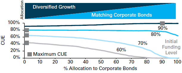
Source: LGIM
On the dark blue line – representing a funding level of 90% – the maximum CUE occurs at an allocation of 90% to corporate bonds. The gives a CUE of around 97%. But the line does not slope upwards significantly. This might indicate that the choice as to whether to have corporate bonds or a diversified growth fund is finely balanced. But what this chart does not show is what happens when the there is a shortfall. If the corporate bonds perform badly, then the outcome is unlikely to be too serious; however, the downside risk with a diversified growth fund is potentially more serious. This does come with greater potential upside, but building up a pension scheme surplus is unlikely to be a key aim for most schemes.
For lower funding levels, the maximum CUE is at 100% in the diversified growth fund. This is because at these levels of funding, even the best possible performance from corporate bonds – that is, absolutely no defaults or downgrades – there will still not be enough assets to meet the liabilities. But this does not mean that a diversified growth fund should be held for self sufficiency; rather, it means that a scheme should aim to improve its funding level to (say) 90%, and to plan for a self-sufficient asset allocation at this point.
Corporate bonds and CUE
So why do corporate bonds look so attractive? Essentially, they offer the opportunity to buy reasonably stable cash flows relatively cheaply. This is because the credit spread includes a number of risk premia that a long-term investor does not necessarily need.
In a self-sufficient pension scheme, corporate bonds are likely to be held on a buy-and-maintain basis. This means that a portfolio is designed to produce cash flows as they are required to meet liabilities, and rebalancing is done only if the credit quality of a particular bond deteriorates.
The credit spread in this portfolio has several components. First, there is the allowance for the expected cost of default and downgrade; second, there is a risk premium, a reward for uncertainty over this cost of default and downgrade; and third, there is a “liquidity premium” – which is essentially a long-term investor premium. These three components are shown below.
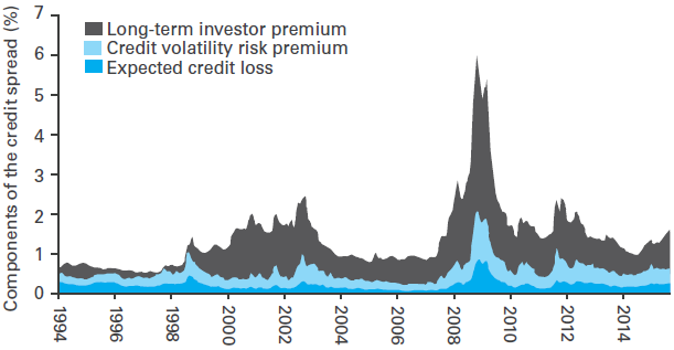
Source: Bloomberg, LGIM
The long-term investor premium is indeed partly a liquidity premium. It is a reward for the fact that it is more costly to trade credit than government bonds, and it can be more difficult. But neither of these factors is a concern for a buy-and-maintain investor.
But the long-term investor premium also includes a reward for spread volatility. This is an issue for an investor having to trade a portfolio regularly, or even having to mark it to market. But a buy-and-maintain investor should care less about volatility in the spread, as long as it does not affect the likelihood of coupons and redemption payments being received. Using an approach like CUE – which looks only at the end point rather than re-assessing solvency on an annual basis – allows credit to be taken for this long-term investor premium.
Consistency with traditional approaches
The CUE can also be linked back to a more traditional valuation approach. The way in which this can be done is as follows. First, decide on the CUE that is regarded as adequate, say 95%. Next, determine the value of assets that would be required to achieve this CUE given the current asset allocation. For example, this might be the value of assets shown in the middle panel of the diagram below, which would give a CUE of 95%. This can be regarded as the value of the liabilities, since if this level of assets were held the scheme would be considered “adequately funded”.
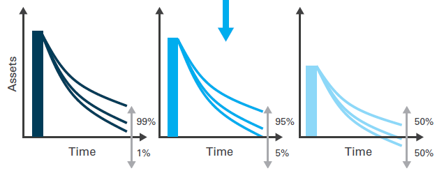
Source: LGIM
Next, this value of liabilities must be used to determine the discount rate implied by the analysis, as shown below. This is done by taking the cash flows and working out what discount rate – perhaps expressed as a spread over the government bonds (Gilts, in this example) – would result in the discounted value of cash flows being equal to the value of liabilities given above. In this way, the implied discount rate can be determined.
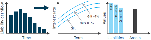
Source: LGIM
Conclusion
CUE seems to offer a more relevant way of measuring funding for a self-sufficient pension scheme. It also allows long-term investor premia in assets such as corporate bonds to be better allowed for. Finally, it can be used to derive a funding level and a discount rate consistent with more traditional approaches – something that might be useful from a regulatory perspective.
*The paper – containing much more detail than this post – can be found here.
![]()